Lean Manufacturing in Action: How to Optimize Line of Balance (LOB) and Productivity Using a Paper Ball Simulation

In the world of manufacturing optimization, transferring complex theoretical concepts from textbook pages to the active shop floor can be a major challenge. How do you teach operators, engineers, and plant managers the critical importance of cycle times, structural bottlenecks, and line balance?

The answer lies in a highly engaging, hands-on industrial engineering training module: The Paper Ball Assembly Line Simulation. By tracking the step-by-step creation of a simple paper ball, teams can visualize exact workflow imbalances, calculate Line of Balance (LOB) and Productivity, and execute concrete optimization strategies.

This practical guide breaks down the full simulation framework, from baseline calculations to advanced continuous improvement options.

Section 1: Process Architecture of the Paper Ball Assembly Line

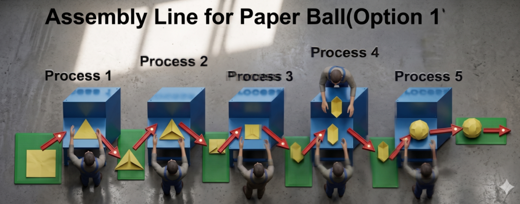
The simulation begins by treating a square piece of paper as raw material, which must flow sequentially through five distinct manual work stations (Processes 1 through 5) to create the finished product.

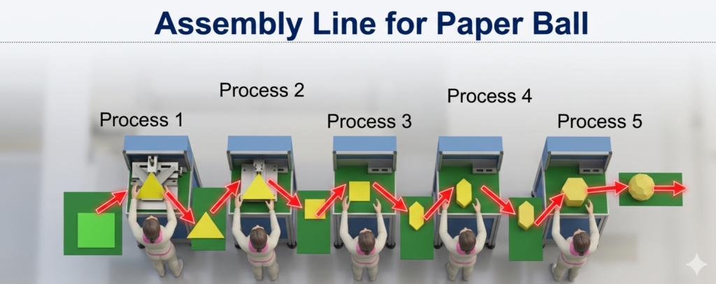
The 5 Standard Operations

1. Process 1 (Making a Triangle): The operator takes the raw square paper and executes the foundational triangular folds.
2. Process 2 (Making a Square): The triangular component is folded inward to form a compact square base.
3. Process 3 (Making a Hexagonal): Advanced multi-axis folds convert the square piece into a hexagonal geometric shape.
4. Process 4 (Inserting Wings): The structural corner flaps (“wings”) are intricately tucked and inserted into side pockets to lock the form.
5. Process 5 (Blowing the Air): The locked unit is expanded into a 3D sphere by inflating it via direct airflow.

Section 2: Diagnosing the Baseline Current State (The Inefficiency Crisis)

To optimize any line, you must establish an empirical baseline. In the initial “Current State” run, Manpower is fixed at 5 operators (1 operator dedicated strictly to each of the 5 processes).

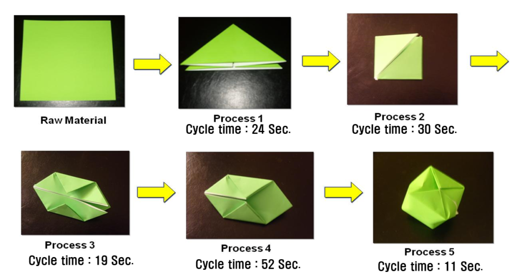
Through close shop floor observation and timing, the individual station cycle times (C/T) are captured as follows:

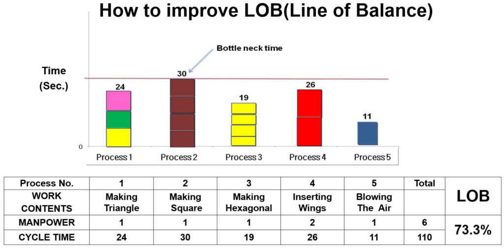
• Process 1 C/T: 24 seconds
• Process 2 C/T: 30 seconds
• Process 3 C/T: 19 seconds
• Process 4 C/T: 52 seconds (🚨 The Structural Bottleneck)
• Process 5 C/T: 11 seconds

Watch the full step-by-step paper ball simulation video on YouTube.

PAPER BALL

The Mathematical Analysis of Waste

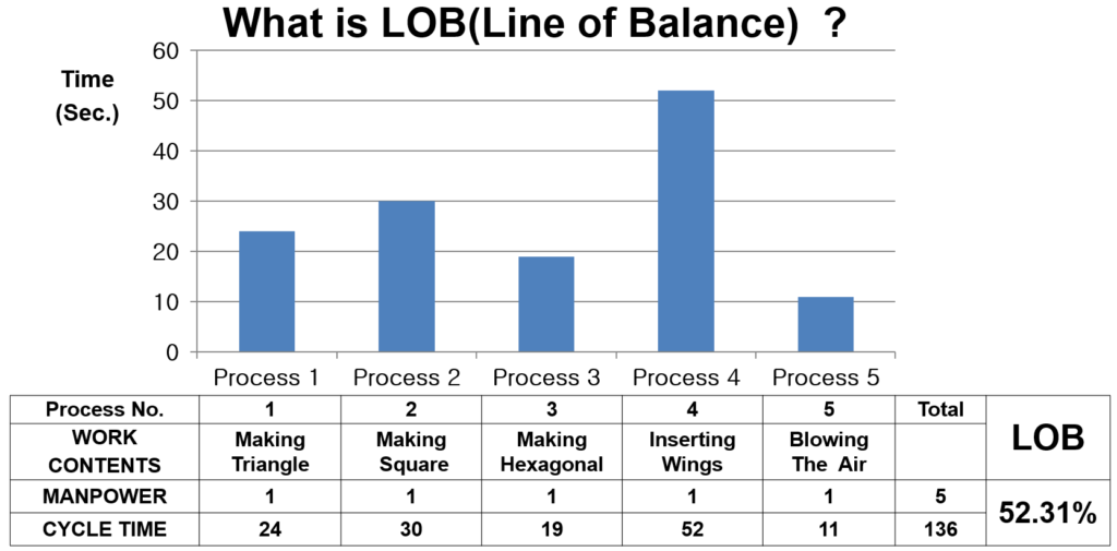
• Total Process Cycle Time (Work Content): 24s + 30s + 19s + 52s + 11s = 136 seconds
• The Bottleneck Time: 52 seconds (Process 4 controls the absolute speed of the entire line).
• Units Per Hour (UPH) Output Capability:

• Baseline Line of Balance (LOB) Rate Calculation:

• Labor Productivity Performance:

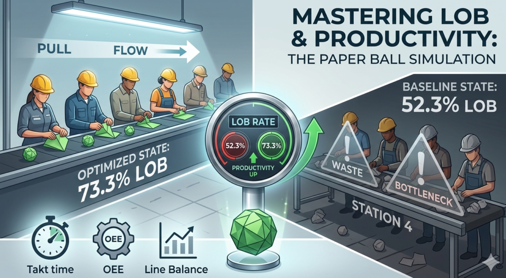
Visual Diagnostic Summary: With an LOB rate of just $52.3%, almost half of the line’s paid labor capital is completely wasted as idle waiting time. Stations 1, 2, 3, and 5 frequently sit starved or blocked because Process 4 takes nearly five times longer than Process 5 to clear a part.

Section 3: The Engineering Strategy — How to Elevate LOB Rates

According to core industrial engineering principles, there are only three mathematical vectors available to drive an upward spiral in line balance efficiency:

1. Reduce the total number of sequential processes via line consolidation.
2. Redistribute the work content to artificially increase total process cycle time across under-utilized operators.
3. Target and reduce the absolute bottleneck time.

Section 4: Operational Optimization (Improvement Option 1)

Let’s apply the third vector by aggressively breaking the bottleneck at Process 4. Since inserting the wings takes a massive 52 seconds due to manual complexity, we introduce a Parallel Workstation Strategy by deploying a second operator directly to Process 4.

This raises our total line Manpower from 5 to 6 operators. By sharing the wing-insertion workload evenly between two parallel stations, the effective cycle time for Process 4 is cut exactly in half:

Recalculating the Improved Post-Optimization State

With the wing-insertion time reduced to 26 seconds, the absolute bottleneck of the assembly line naturally shifts to Process 2 (Making a Square) at 30 seconds.

Let’s look at the mathematical results of this single modification:

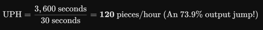
• New Line Bottleneck Time: 30 seconds
• New UPH Output Capability:

• Optimized Line of Balance (LOB) Rate:

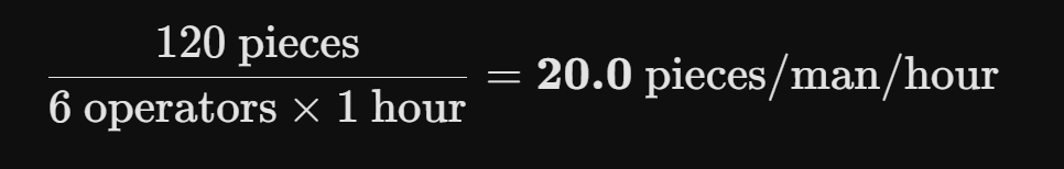
• Optimized Labor Productivity Performance:

Section 5: Comparative Performance Dashboard

By comparing the performance metrics side by side, we can clearly see the massive impact of using data to drive line adjustments:

Operational Metric	Current Baseline State	Optimized State (Option 1)	Performance Variance
Total Line Manpower	5 Operators	6 Operators	+1 Headcount
Line Bottleneck Time	52 Seconds	30 Seconds	-22 Seconds (Faster Pace)
Hourly Output (UPH)	69 Pieces / Hour	120 Pieces / Hour	+73.9% Throughput
Line of Balance (LOB%)	52.3%	73.3%	+21.0% Balance Efficiency
Labor Productivity	13.8 Pcs/Man/Hr	20.0 Pcs/Man/Hr	+44.9% Efficiency Gain

Section 6: Lean Kaizen Challenge — Driving Further Innovation

While Option 1 successfully elevated productivity to 20 pieces/man/hour, a true continuous improvement practitioner never stops searching for hidden wastes. Ask your training teams the following core questions to push for further optimization:

1. Can we cross-train operators to implement a “Chaku-Chaku” (Load-Load) cell? Notice that Process 5 (Blowing Air) takes only 11 seconds, and Process 3 (Hexagonal) takes only 19 seconds. Combined, their work content equals exactly 30 seconds ($19s + 11s$). By combining these tasks under a single multi-skilled worker, can we eliminate one operator entirely while maintaining our 30-second pace?
2. Can we apply SMED/Ergonomics to Process 4? Instead of automatically adding a 6th worker, can we redesign the folding fixtures or create simple manual creasing jigs to lower the 52-second cycle time down to 30 seconds through motion efficiency alone?

Section 7: Advanced Line Balancing: Maximizing LOB and Productivity Through Work Element Breakdown

As shown in the chart below, this advanced optimization method focuses on breaking down individual tasks within each process and redistributing those micro-work elements to other under-utilized stations.

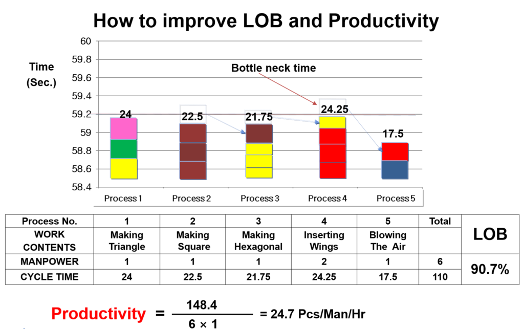
By meticulously reallocating the workload across the 5 stations, the line bottleneck time is significantly minimized down to 24.25 seconds at Process 4. This granular balancing strategy successfully eliminates structural idle time, driving the Line of Balance (LOB) efficiency rate to an impressive 90.7%. Consequently, total labor productivity sees a substantial leap, achieving 24.7 Pcs/Man/Hr with the same 6-man team configuration.

Conclusion: Turning Simple Simulations into Factory Floor Success

The paper ball simulation proves that maximizing plant productivity isn’t about forcing operators to work faster—it’s about using industrial engineering math to balance out work distribution and remove structural layout bottlenecks.

Bring this simulation into your next continuous improvement workshop, capture your live metrics, and watch your operators transform raw data into optimized line balance.

For an step-by-step visual walkthrough of this folding sequence and to see this layout in action on the training floor, check out the official demonstration video on our YouTube Channel!

🔗 Recommended Reading:

7 Wastes or 5S post here :7 Wastes : The Definitive Guide to Eliminating Non-Value-Adding Activities

PDCA Problem Solving here : The Power of the PDCA Report in 4 Steps